Five Coupled Models
Multi-model integration — our core strength.
Each model feeds the next, while also informing the previous. Combined, they deliver an integrated assessment that no single model can provide on its own.
We use 3D ray tracing to simulate light availability across the full field footprint — calculating PAR, DLI, and shadow distribution from panel geometry, tilt, azimuth, and local sun angles. The result is a spatial map of crop-usable light (%) relative to open-field conditions, resolved by agronomic zone. This forms the foundational input for all subsequent model steps.
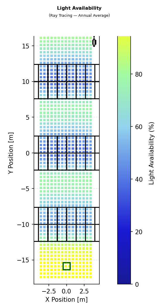
Light availability map — growing season average. Min: 27.5%, Max: 79.5%, Mean: 57.4%.
Solar panels alter the thermal environment of the crop canopy. We model soil temperature, humidity, and air movement across field zones — quantifying how conditions differ beneath the modules, between rows, and within the farming zone relative to open-field reference conditions. These microclimate deltas directly inform crop water demand, heat stress risk, and frost exposure in the models that follow.
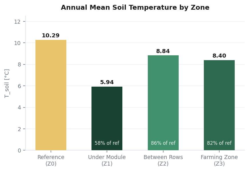
Annual mean soil temperature by zone — under-module zones show measurable cooling.
Panels intercept rainfall and alter evapotranspiration. Using soil-water models, we simulate actual evapotranspiration (AET) by zone across the full year — quantifying shifts in crop water use, drought stress risk, and irrigation demand. Monthly AET comparisons between agrivoltaic and open-field scenarios can be translated directly into irrigation cost deltas for water-managed crops.
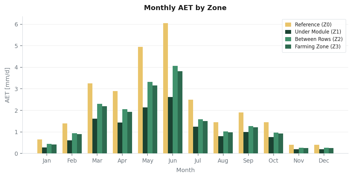
Monthly AET (mm/d) by zone — panels reduce water demand under-module.
We run crop growth models driven by the modified light, microclimate, and soil-water inputs from Steps 1–3. Results are cross-validated against our crop studies database using statistical regression, producing a probability-weighted range — expected, upside, and downside — rather than a single-point estimate. Where available, outputs are also checked against and calibrated using remotely sensed LAI and historical field performance at site level.
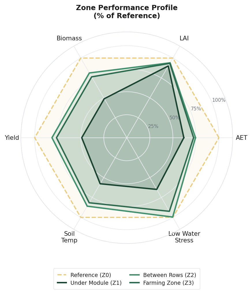
Zone performance profile (% of reference) — LAI, AET, biomass, yield, soil temperature, water stress.
Agricultural viability depends on whether the farm can actually be operated. Our proprietary model assesses machinery clearance, row accessibility, additional fuel use, time efficiency, and whether equipment can operate effectively under the proposed system geometry. This step surfaces operational constraints before construction and feeds directly into design optimization.
Outputs include minimum clearance heights, row width requirements, turning radii, and seasonal access windows — per machinery type and crop operation.
Not every agricultural risk can be captured quantitatively. That is why all model outputs are reviewed by an agronomist, who interprets the results in the context of the crop, field conditions, and farming system. This qualitative step helps identify practical risks and considerations — such as pest pressure, disease sensitivity, waterlogging risk, and other site-specific management constraints — that may affect real-world performance.